In my previous article I provided a sketch of the light detection process in a modern CMOS camera, from photo quants (photons) to digital numbers. We discovered two important physical parameters quantum efficiency qν and camera gain gPC that describe the light detection process in a digital CMOS camera. This monthly notice will focus on how we can evaluate how many photo electrons are detected from the digital numbers in an astronomical picture recorded. Unfortunately, physics and astronomy won't work without mathematics, but computations aren't too hard.
What is unity gain?
Camera gain gPC describes the relation between the number of photo electrons collected and the digital pixel intensity values. In case of a typical scientific or dedicated astronomical camera, whether cooled or not, user control by software provides means to select between arbitrary gain values. Conventional photo cameras provide a knob to select between ISO settings, that define the gain to increase pixel values from a picture taken at low light level conditions. Unity gain denotes the gain setting gPC, where the digital unit of the pixel value is equal, or at least closest to the number of photo electrons freed by photons within the silicon device. Camera gain is simply the quotient of digital numbers divided by the number of electrons counted. If camera gain gPC is smaller than one, then the number of electrons counted are larger than the digital units in the recorded image. If gPC is larger than one, then the digital numbers in our image express to have found more electrons than actually measured.
gPC ≈ 1.
Ideally, camera gain gPC shall be approximately one. This is the unity gain condition.
Evaluation of unity gain
Certain manufacturers of astronomical imaging devices provide information about the gain value, that is closest to the condition. For conventional photo camera ISO settings that reflect unity gain are available from internet databases (see literature section). However, if precise measures are required, the exact gain setting for a specific camera, which is closest to the unity gain condition, shall be evaluated by conducting experiments with different gain settings.
Variance is a mathematical term, that is defined as the mean squared difference of random values and mean value. As already outlined in my previous article, for Poisson distribution the mean value E[X] of the pixel intensities X recorded is the same as their variance Var(X). This can be written as:
E[X] = Var(X)
or rewritten
1 = E[X] / Var(X)
If the photon count is multiplied by an arbitrary factor gPC, mean value and variance of the noisy numbers will not satisfy the above condition. In this case we can compute gPC from the invers quotient of mean value and variance to establish the relation between digital numbers and photo count.
gPC = Var(X) / E[X]
The other way round, we can compute a direct estimate for the electron count from dividing digital numbers in the image by gPC.
To simplify things for further discussion we will check, which gain setting satisfies the above Poisson noise condition, where the quotient of mean value and variance will be closest to one. This can be evaluated by collecting exposures taken from a flat screen at different gain or ISO settings. In astronomy a set of sky flatfield exposures taken at different gain settings is a perfect choice. Under the assumption, neighbouring pixels shall have equal quantum efficiencies, single sky flatfield frames taken at different ISO settings enable a quick evaluation where one shall expect unity gain condition. The assumption is certainly valid for most imaging sensors that provide homogeneous illumination results with no big variation of quantum efficiency across pixels. However, one shall carefully select a homogeneously illuminated pixel area close to the maximum intensity, found with no gradient, which is typically close to the center of the flatfield exposure. Also exclude portions with dust particles or dead pixels that will introduce large scatter of intensities. Finally, we compute mean value E(X) and variance Var(X) of the pixel intensities recorded. Plot values into a graph and see which ISO or gain setting will reflect unity gain the best.
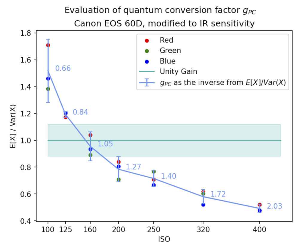
Figure 2: Plot of the quotient E[X]/Var(X) and its inverse quantum conversion factor gPC obtained from pixel intensities that are found in an area of 25x25 pixel of individual sky flatfield frames taken at different ISO settings. A Canon EOS 60D camera was used for this experiment, that has been "astro-modified" by removal of the UV/IR cut filter and diffusor in front of the sensor. Plotted are the measured values for each red, green and blue color channel. Computations take into account, that two green pixel form the digital signal of a Bayer matrix imaging device.
The above plot indicates ISO 160 is closest to satisfy the Poisson noise condition using mean value and variance. This is the point, where unity gain is achieved and the arbitrary gain factor gPC is almost equal to one. If you ever read discussions, what ISO setting will be beneficial to astrophotography, or more ambitious applications like stellar photometry the plot reveals an interesting result. Settings in the range from ISO 200 onwards to ISO 400 and higher will provide more gain to the signal, but no additional information in terms of having counted more photo electrons.
Are the very high gain (ISO) settings beneficial to astrophotography?
The answer is: No.
With ISO settings larger than unity gain, like ISO 200 or ISO 400, digital numbers in the image start to represent a fraction of a single photo electron collected. However, as with any other quantum particle in physics, a photo electron cannot be split or divided into fractions of itself! How could this happen? Camera gain happens at the electronic amplifier stage in our camera sensor. Numbers digitized at any ISO settings represent any arbitrary integer number of electrons amplified by the arbitrary gain, not a number of actual photons counted. Additional readout noise will add to the images, which makes noise distribution more broader at high ISO settings. Numbers stored in the digital image start to appear like a fraction of a photon event, because the electronics amplifies arbitrary electron current measured, that represents a fractional probability to have detected a photon event multiplied by the amplification factor. This is not any exact integer number of electrons or photo events detected.
What about read-out noise?
You may have read about recommendations from amateurs to use high gain settings, like ISO 1600 or more for digital astrophotography using CMOS DSLRs or mirror-less digital cameras. This is claimed to increase the distance between read-out noise and signal noise level. Numbers recorded in a digital image may lie about the true nature and actual count of the quantum particles, i.e. the number of real photon events detected by the sensor pixel. Gain settings beyond ISO 200 will amplify a noisy number, but will not unveil more light from the noisy signal. In fact there are indications, that the level of read-out noise vs. signal can be even enlarged by higher ISO settings. On the other hand, the intrinsic natural photon noise from the low sky background level has to be overcome to increase the detection limit of a faint astronomical light source above sky background. Modern astronomical CMOS imaging sensors and commercial DSLRs or mirror-less digital cameras operate at photon-counting level with a very low read-out noise of typically 3 electrons per pixel or less! This is already in the order of or less than the standard deviation of typically few electrons counted in V bandpass from the natural illumination of the night sky. Suburban skies provide much more light and thus much more noise from the sky background. As a side note, the use of modern CMOS imaging devices is different from using classical CCD imaging sensors, that suffered from larger system noise levels and non-linearities.
My recommendation to astrophotographers: Do not push ISO settings far beyond unity gain to avoid empty amplification of the photon count. In the example ISO 400 of a real Canon camera corresponds to a gain factor where one digital unit represent "half a photo electron" counted. The consequence of using high gain settings is loss of dynamic range. A digital camera has a limited range of digital numbers. Typically this is 14 bit resolution for modern DSLR cameras with a digital value range between zero and up to a maximum possible digital value of 16383. That means a bright star will run into saturation sooner due to early cut-off from the analog-digital converter. So there exist useless ISO settings, that should be expected earlier, than thought. High ISO settings do not provide an increase of light signal from the recorded digital pixel intensities.
From the many observations over years, I suggest using ISO 400 instead of ISO 160 seems reasonable. Again, this means loss of about one apparent magnitude at the upper intensities of bright stars recorded in the image. Higher ISO setting do not provide any benefit, but limit dynamic range. Deep sky imaging uses image stacking techniques. Image stacking can be impacted by static hot pixels, that will develop with longer exposure times. Certain experiments indicate hot pixels are more dominant at lower ISO settings for a DSLR. This is different from cooled astronomical imaging devices. The physics and nature behind hot pixels in CCD or CMOS imaging sensors is still not well understood and shall not be discussed further in this article. Operating a Canon DSLR at ISO 400 is a good compromise between the trade-off of limiting dynamic range at a reasonable low noise level.
Conclusion and outlook
We should not push gain settings of DSLRs too far. The same applies to dedicated astronomical cameras, which typically are used at unity gain or even lower gain settings. Such astronomical devices taken as an example, it also does not seem reasonable to operate DSLRs at much larger gain settings. At ISO 160 my Canon camera already operates counting single photons per digital unit. This is well supported by indepent research (see also "Photons to photos internet database" link below). ISO 400 seems a reasonable compromise between limiting dynamic range by cutting off light from brighter stars, optimal readout noise and minimizing any impact from hot pixels in the digital image.
In my next article I will move on and discuss the relationship between flux and apparent magnitude. The Vega photometric system will be the next milestone to understand the relationship between (stellar) magnitudes and photo flux.
Literature
- Planck, M., 1901. On the Law of Distribution of Energy in the Normal Spectrum. Annalen der Physik. vol.4, p.553
- Bauer, T., Efficient Pixel Binning of Photographs. IADIS International Journal on Computer Science and Information Systems, vol. VI, no. 1, p.1-13, P. Isaías and M. Paprzycki (eds.), 2011. ISSN: 1646-3692
- Photons to photos internet database: https://www.photonstophotos.net/Charts/RN_e.htm